
Two things the enterprise AI world hasn’t fully woken up to yet:
First — F500 enterprises setting up a dedicated GPU cluster with a custom-trained model for targeted use cases, running alongside frontier closed model like Claude Opus 4.6, is a business model the frontier labs haven’t fully explored. The labs still own the model and weights. The enterprise owns the security and data sovereignty layer. That’s a powerful, underexplored wedge.
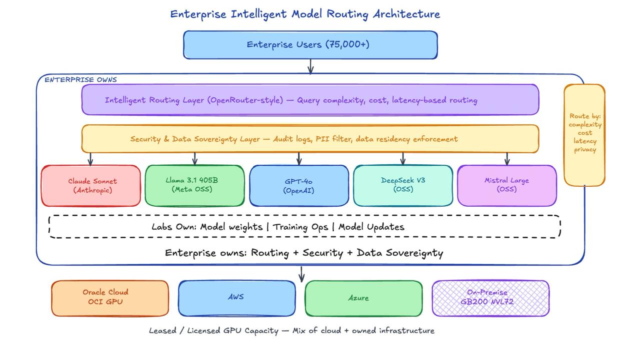
Second — most enterprises have an untapped ability to build an intelligent routing layer on top of multiple models hosted by leading cloud providers like Oracle. Think OpenRouter sitting on top of 4–5 models leased or licensed by the enterprise — a mix of closed and open source. This intelligent routing layer is the enterprise superpower that almost no one is building yet.
Both of these ideas rest on the same foundation: understanding what inference actually costs at scale. Not training. Inference. The part nobody budgets correctly until they’re hemorrhaging GPU hours and wondering why their SLOs are on fire.
This post is the infrastructure reckoning. By the end, you’ll know exactly why inference is hard, what drives the costs, and how to think about building an enterprise AI stack that doesn’t blow up in production.
Why Inference ≠ Training
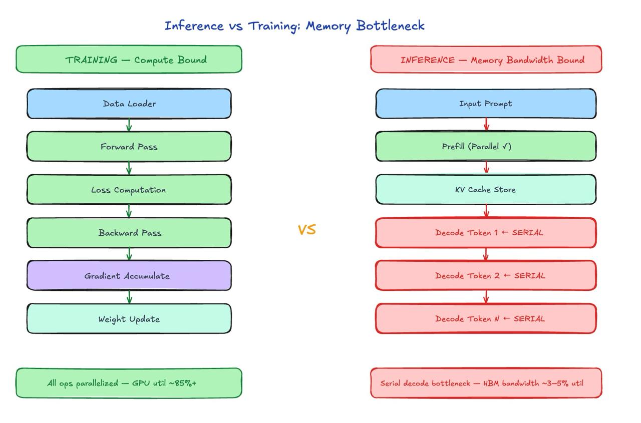
The GPU bills that made headlines were training bills. But inference is where you spend forever — every user request, every API call, every production query. And inference has a fundamentally different bottleneck than training.
Training is compute-bound. You’re doing massive matrix multiplications across huge batches. Your GPU’s tensor cores are saturated. Arithmetic intensity is high. FLOP utilization is the constraint.
Inference is memory-bandwidth-bound. At batch_size=1 (which is what most requests look like at the token level), you’re loading billions of parameters from HBM just to do a tiny multiply-accumulate for each generated token. The math is trivial. The bottleneck is how fast you can stream weights from memory to compute.
The autoregressive decode loop makes this worse. Each token depends on every previous token — you cannot parallelize across the sequence. You’re locked into a serial process: load weights → compute one token → append to KV cache → repeat. This is the fundamental architecture of transformer inference, and no amount of clever scheduling changes the serial nature of decoding.
Add SLO pressure to this. Enterprise users expect <500ms time-to-first-token (TTFT) and >30 tokens/sec generation throughput. These are not negotiable if you’re building a product. They’re also in direct tension with each other — batching more requests improves throughput but kills latency. This tradeoff is what keeps inference engineers up at night.
The Context Window Explosion: 2K → 1M Tokens
GPT-2 launched with 1,024 token context. GPT-3: 2,048. GPT-4: 8K, then 32K, then 128K. Gemini 1.5 Pro: 1 million tokens. Claude 3.7: 200K.
This is a 500x expansion in five years. And every single one of those tokens needs to live in memory during inference.
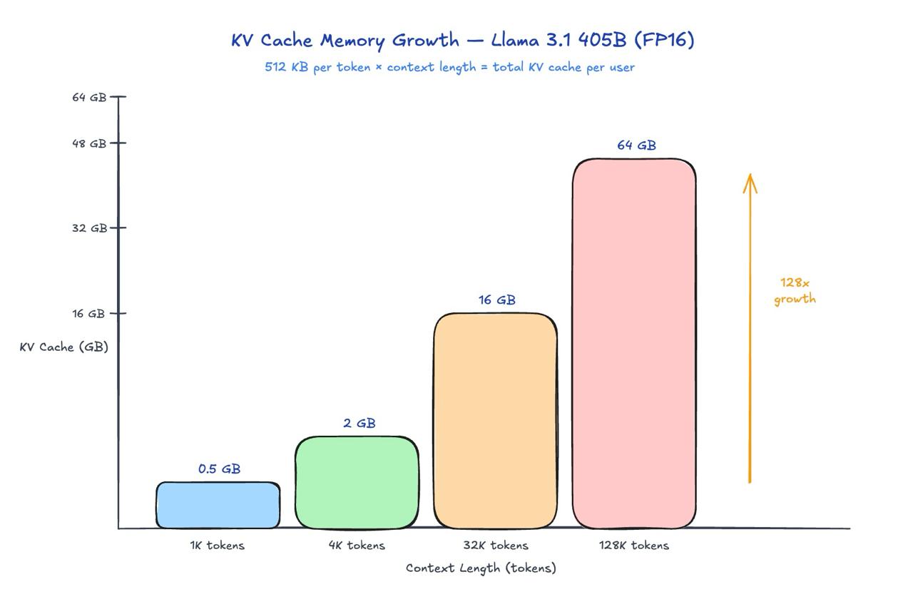
The KV(key-value) cache — the structure that stores the key and value tensors for all previous tokens so you don’t recompute attention from scratch — scales linearly with context length. For a large model like Llama 3.1 405B, a single user session at 128K context consumes 64 GB of GPU memory. Not for the model weights. Just for one conversation’s history.
Context window is where the contextual awareness for the given task at hand is important for. A small context window means either you have a model post-trained for an extremely focused task like front-end design, or for generic models(where th
it means the model quickly loses context.
This is why context window size is not just a product feature. It’s an infrastructure commitment. Every 4x increase in max context is a 4x increase in KV cache memory pressure per concurrent user. At enterprise scale with thousands of concurrent sessions, this is where GPU clusters break.
KV Cache Deep Dive: The Math That Explains Everything
The KV cache is the single most important concept to understand in production LLM inference. Get this wrong and everything downstream — GPU sizing, concurrency planning, SLO design — is wrong too.
What the KV cache actually is
Transformers use self-attention: every token attends to every previous token to decide what information to carry forward. To compute attention for token N, you need the Key and Value vectors for tokens 1 through N-1. Recomputing them from scratch every step is O(N²) work per token — catastrophically expensive at long contexts.
The KV cache solves this by storing those Key and Value vectors in GPU memory after they’re first computed. Each new token just appends its K and V to the cache, then reads the whole cache to compute attention. This brings decode-step cost from O(N²) to O(N) — but it trades compute for memory. And at the scale of modern models and context windows, that memory bill is enormous.
Where it sits in the inference flow
Every inference request goes through two distinct phases:
- Prefill: The entire input prompt is processed in one parallel forward pass. All K and V vectors for the input tokens are computed and written to the KV cache. This is compute-intensive (the GPU loves it), and the KV cache starts empty and fills to input_length × 512 KB per layer.
- Decode: One token is generated per step. Each step reads the entire KV cache, computes attention against all previous tokens, generates the next token, then appends its K and V to the cache. The cache grows by 512 KB with every single token generated. This phase is memory-bandwidth-bound — not because the math is hard, but because reading a potentially multi-GB cache from HBM every step is the bottleneck.
This is the fundamental split that makes inference infrastructure design non-obvious: prefill and decode have completely different hardware profiles. Prefill wants compute; decode wants memory bandwidth. Running them on the same GPU is a compromise that neither optimizes.
The math (Llama 3.1 405B at FP16)
KV cache per token:
  = 2 (K and V) × num_kv_heads × head_dim × bytes_per_element × num_layers
  = 2 × 8 KV heads × 128 head_dim × 2 bytes (FP16) × 128 layers
  = 524,288 bytes
  = 512 KB per token
At a typical p90 context of 4,608 tokens (4K input + 512 output), each concurrent user needs 2.25 GB of KV cache memory. 6,000 concurrent users? That’s 13.5 TB. Just for KV cache. On top of 810 GB for model weights.
Why 6000 users? – because we are trying to understand inference, which happens at scale when we hit the OpenAI and Anthropic API’s. So 6000 is my typical enterprise scale assumption, bleeding edge AI adopters!
This is the number that breaks naive infrastructure plans.
Why KV cache dominates production infrastructure decisions
The model weights are a fixed cost — 810 GB loaded once, shared across all requests. KV cache is a per-request variable cost that scales linearly with both context length and concurrency. At low concurrency, weights dominate. Scale up users or context length and KV cache becomes the binding constraint long before compute does.
Three practical implications that routinely surprise teams:
- Long context is an infrastructure commitment, not a product feature. Enabling 128K context doesn’t just improve UX — it multiplies per-user GPU memory cost by 32× compared to 4K context. You can’t just flip a flag.
- Concurrency is bounded by memory, not compute. A GB200 cluster with 27 TB of VRAM can support ~12,000 concurrent 4K-context sessions (after weights). Extend that to 32K context and you’re down to ~1,500 concurrent sessions on the same hardware. Same GPUs, 8× fewer concurrent users.
- Eviction policy matters at enterprise scale. When GPU memory is full, you have to evict KV cache entries — either dropping users or swapping to CPU RAM (slow). vLLM’s paged attention delays this by eliminating fragmentation, but you still need explicit policies for what happens under sustained peak load.
The two innovations that made it manageable
Paged Attention (vLLM): Borrowed from OS virtual memory, paged attention breaks the KV cache into fixed-size blocks (pages) that don’t need to be contiguous in GPU memory. Before this, systems pre-allocated the maximum possible KV cache for each request — a 128K-context request reserved 64 GB even if it only used 2K. Memory utilization was abysmal. Paged attention achieves near-zero waste and enables efficient memory sharing between sequences. This is why vLLM changed production inference — not just the engineering, but the economic model.
Prefix Caching: When multiple requests share a common prefix — system prompt, few-shot examples, a long document being queried repeatedly — the KV cache for that prefix can be computed once and reused across requests. For enterprise deployments with a 2K-token system prompt shared by all users, prefix caching eliminates that 1 GB of recomputed KV cache work on every single request. At 780 QPS, that’s the difference between sustainable and untenable compute bills. Prefix caching hit rates of 60–80% are common in enterprise deployments with consistent system prompts.
I feel all my experience writing memory-optimised code for 8-bit to 64-bit microcontrollers in early parts of my career is helping me to get my head around the limitations of compute and memory requirements. Coupled with my experience of developing cloud native applications in building scalable and resilient internet applications, helps me to connect the hardware and software worlds that AI applications are trending towards. What a world to live in.
Batching Strategies: From Naïve to Continuous
Static batching is what you get if you don’t think about inference: collect N requests, run them together, return results. Simple, clean, terrible. Requests with short outputs force long ones to wait. GPU utilization craters whenever batch composition is uneven.
Continuous batching (also called in-flight batching or iteration-level scheduling) fixes this. Instead of waiting for all sequences in a batch to finish, new requests are inserted into the batch the moment a slot opens up. Throughput improvements of 5–23x over static batching in benchmarks. This is now table stakes in any production inference stack.
Prefill/decode disaggregation is the next frontier. Prefill (processing the input prompt) is compute-intensive and can be highly parallelized. Decode (generating output tokens) is memory-bandwidth-bound and serial. Running them on the same hardware is a compromise. Disaggregation splits them onto different GPU pools — prefill on compute-dense hardware, decode on memory-bandwidth-optimized hardware. Early benchmarks show 2–3x throughput improvements with dramatically lower TTFT at high load.
Model Parallelism: Splitting 405B Across GPUs
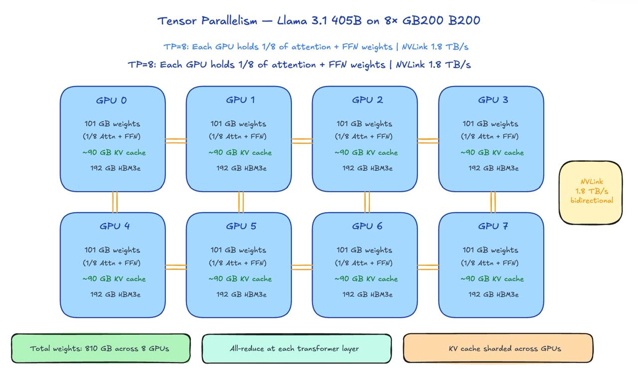
A 405B parameter model at FP16 is 810 GB. No single GPU holds that. You need parallelism — but which kind?
Tensor Parallelism (TP): Split individual weight matrices across multiple GPUs. Each GPU holds 1/N of every attention head matrix and FFN layer. All-reduce operations synchronize partial results at each layer. High communication overhead — requires NVLink (1.8 TB/s) to be practical. TP=8 is the sweet spot for most large models: each GPU gets 101 GB of weights, leaving ~90 GB headroom for KV cache. Beyond TP=8, communication overhead starts eating into gains.
Pipeline Parallelism (PP): Split layers across GPUs — GPU 0 handles layers 1–32, GPU 1 handles 33–64, etc. Lower communication overhead than TP (only activations pass between stages, not partial weight results). But introduces pipeline bubbles: GPUs sit idle while waiting for the previous stage to finish. PP works well for training (large micro-batches fill the pipeline) but is less elegant for inference where batch sizes are small and latency matters.
In practice: Production inference uses TP within a server node (connected by NVLink) and PP across nodes (connected by InfiniBand). The GB200 NVL72 rack with 72 GPUs connected by NVLink at 1.8 TB/s is designed exactly for this — run TP=8 across 8 GPUs within a group, then PP across groups.
Quantization: The Memory Compression Lever
Quantization reduces the numerical precision of model weights and activations, trading a small accuracy hit for massive memory and speed gains.
For a 405B parameter model:
| Precision | Bytes/Param | Model Size (405B) | GPUs Needed (192 GB) | Quality Impact |
|---|---|---|---|---|
| FP32 | 4 | 1,620 GB (1.62 TB) | 9+ | Baseline |
| FP16 / BF16 | 2 | 810 GB | 5 (practical: 8) | Negligible |
| INT8 | 1 | 405 GB | 3 (practical: 4) | Minor on most tasks |
| INT4 (GPTQ/AWQ) | 0.5 | ~202 GB | 2 | Noticeable, task-dependent |
| FP8 | 1 | 405 GB | 3 (practical: 4) | Near-negligible with calibration |
FP8 is the practical sweet spot in 2025: GB200’s H200 successor supports native FP8 tensor cores, delivering near-FP16 quality at INT8 memory footprint. The GB200 B200 GPU pushes ~50K tokens/sec at FP8 vs ~25K at FP16 — a 2x throughput gain that can mean the difference between 4 racks and 8 racks in your infrastructure plan.
The Inference Engine Landscape
Three engines dominate production LLM inference in 2025:
vLLM — Open source, Python-first, and the de facto standard for most deployments. Pioneered paged attention and continuous batching. Broad model support, active community, straightforward deployment. If you’re starting fresh and need proven production infrastructure, start here. Limitation: Python overhead can cap throughput at extreme scales.
TensorRT-LLM (NVIDIA) — NVIDIA’s inference optimizer, purpose-built for their hardware. Compiles models into optimized CUDA kernels, supports FP8/INT4/INT8, implements tensor parallelism natively. Delivers the highest raw throughput on NVIDIA hardware, but requires NVIDIA’s ecosystem and significantly more engineering effort to customize. The right choice when you’re going all-in on NVIDIA and need to squeeze the last 30% of performance.
SGLang — The newest entrant and arguably the most interesting. Built around “structured generation” — efficiently handling complex LLM programs with branching, tool use, multi-turn interactions, and constrained generation. Outperforms vLLM on workloads with complex control flow. If your enterprise use case involves agents, chains, or structured outputs (most do), SGLang deserves a benchmark slot.
Honorable mentions: Ollama for developer-local inference, LMDeploy for quantization-heavy deployments, Triton Inference Server for multi-model production environments.
Sizing a GB200 Cluster for 75,000 Enterprise Users: The Math
Let’s make this concrete. Llama 3.1 405B at FP16. 75,000 enterprise users. Here’s the full sizing exercise.
A) Weight Memory
405B parameters × 2 bytes (FP16) = 810 GB total weight memory

GB200 B200 GPU: 192 GB HBM3e
Minimum GPUs for weights alone: ⌈810 / 192⌉ = 5 GPUs

Practical TP=8 configuration:
  810 GB / 8 GPUs = 101.25 GB weights per GPU
  192 GB - 101.25 GB = 90.75 GB headroom per GPU (for KV cache)
B) KV Cache Per User
KV cache per token = 2 × 8 KV heads × 128 head_dim × 2 bytes (FP16) × 128 layers
                   = 524,288 bytes = 512 KB/token

p90 context: 4,096 input + 512 output = 4,608 tokens per session
KV cache per concurrent user = 4,608 × 512 KB = 2.25 GB
C) Peak Concurrency
75,000 users × 8% concurrency = 6,000 concurrent sessions
Total KV cache = 6,000 × 2.25 GB = 13,500 GB = 13.5 TB
D) Total VRAM Required
810 GB (weights) + 13,500 GB (KV cache) + 20% overhead = ~17.2 TB total VRAME) GB200 NVL72 Rack Sizing
- Each NVL72 rack: 72 GPUs × 192 GB = 13,824 GB ≈ 13.5 TB VRAM
- Minimum viable: 2 racks (~27 TB — covers weights + full 6K concurrent KV cache with headroom)
- Production recommendation: 3 racks (adds redundancy + headroom for 128K context bursts)
- Cost estimate: ~$10–15M per rack → $30–45M for production cluster
F) Throughput Math
75,000 users × 150 queries/day = 11.25M queries/day
Peak 8-hour window: 11.25M / 28,800 seconds = 390 QPS average, ~780 QPS at p90

GB200 rack throughput: ~50K tokens/sec (FP8), ~25K tokens/sec (FP16)

At avg 512 output tokens/query:
  780 QPS × 512 tokens = 400K tokens/sec needed

For pure FP16 throughput: 400K / 25K = 16 racks needed
With FP8 + aggressive batching: reduces to 4–6 racks
G) Final Recommendation
| Configuration | Racks | Approach | Cost | Verdict |
|---|---|---|---|---|
| Minimum Viable | 2 | FP16, 6K concurrent KV cache | $20–30M | Fits model + memory, constrained throughput |
| Production | 4 | FP8 + batching, 780 QPS | $40–60M | Handles peak throughput with redundancy |
| INT8 Alternative | 2 | INT8 weights (405 GB) + KV cache headroom | $20–30M | Same cost, better memory efficiency |
The bottom line: A production-grade private deployment of Llama 3.1 405B for 75,000 enterprise users costs $40–60M in hardware alone, before power, cooling, networking, and ops. This is not cloud economics — this is HPC economics. And it’s exactly why the intelligent routing model (see conclusion) is often the smarter play.
GPU Infrastructure Implications
Beyond raw GPU count, enterprise inference at scale requires infrastructure decisions that most teams underestimate:
Networking: Tensor parallelism across GPUs requires near-NVLink bandwidth. Within a GB200 NVL72 rack, NVLink at 1.8 TB/s handles intra-rack TP traffic. Cross-rack communication requires InfiniBand HDR/NDR at 400–800 Gbps. Undersized networking creates bottlenecks that no amount of GPU compute can fix.
Power and cooling: Each GB200 NVL72 rack draws ~120 kW. Four racks = 480 kW. Most enterprise data centers max out at 10–20 kW per rack. GB200 deployments require purpose-built facilities with liquid cooling. This is not a footnote — it’s a 6–12 month procurement and construction timeline before your first GPU comes online.
Reliability architecture: At 4 racks of 72 GPUs each, you have 288 GPUs. GPU failures at this scale are not edge cases — they’re scheduled events. Your inference stack needs graceful degradation, automatic failover, and the ability to reroute traffic when a rack or node goes down. This means Kubernetes orchestration, health checks, and a control plane that understands GPU topology.
The cloud alternative math: AWS, Oracle, and Azure offer on-demand and reserved GPU capacity. Oracle’s OCI is particularly aggressive on pricing for enterprise AI workloads. At $10–15/hour per H100 equivalent, a 576-GPU equivalent (8 racks, FP8) runs ~$5.7M/month at on-demand pricing, or ~$2–3M/month on 3-year reserved. Compare that to $40–60M CapEx plus ops costs — the crossover point for owned infrastructure is typically >3 years of heavy utilization. Below that, cloud is usually cheaper when you account for TCO honestly.
The Enterprise Play: Data Sovereignty + Intelligent Routing
Here’s where we come back to the contrarian frame that opened this post.
The math above — $40–60M for owned infrastructure — looks daunting. But framed correctly, it’s a data sovereignty acquisition.
The enterprise doesn’t buy GPU clusters to compete with OpenAI. They buy them to guarantee that their proprietary data, their customer conversations, their IP never touches a shared cloud inference environment. The model weights stay with the lab. The security perimeter and data layer are owned entirely by the enterprise.
This is an underexplored split that frontier labs haven’t aggressively productized: lab owns the model, enterprise owns the infrastructure and data sovereignty. Claude Sonnet 4.5 fine-tuned for financial services, running on Oracle Cloud dedicated GPU capacity, with all data staying within the enterprise’s network boundary — that’s a defensible product that no SaaS vendor can replicate.
The second play is even more interesting for enterprises that don’t need frontier-scale inference for every query. Most enterprise AI workloads don’t require a 405B parameter model. A 70B model handles 80% of queries adequately. A 7B model handles 40%. An intelligent routing layer — built on top of 4–5 models licensed across Oracle Cloud, AWS, and Azure — can make these decisions dynamically: route simple queries to cheap models, complex reasoning to frontier models, sensitive data to on-premises deployments.
Think OpenRouter, but enterprise-owned, with full audit trails, cost controls, and the ability to mix open-source models (Kimi K2.5, Qwen 3.5, MiniMax, Llama, Mistral, DeepSeek V3) with closed commercial APIs (Claude, GPT-4). The routing logic becomes a core enterprise competency, not a vendor’s feature.
The infrastructure knowledge in this post — KV cache math, batching strategies, quantization tradeoffs, parallelism configurations — is exactly what you need to design that routing layer intelligently. Routing based on query complexity requires understanding what makes a query compute-intensive. Choosing the right model for context window requirements requires knowing what KV cache costs. Setting SLOs requires understanding the latency/throughput tradeoff.
The enterprises that win in the next 3 years won’t be the ones who buy the most GPUs. They’ll be the ones who understand inference well enough to build intelligent infrastructure on top of existing capacity — owned, leased, or cloud — and route every query to the right model at the right cost.
That’s the infrastructure reckoning. The math is hard. The hardware is expensive. But the leverage available to enterprises who understand it is enormous — and mostly untapped.